D. Schluter, University of BC
Fit models to data
This page provides tips and recommendations for fitting linear and nonlinear models to data. Updated and revised frequently (click the reload button on your browser to make sure you are seeing the most recent version).The main model-fitting commands covered on this page are:
lm(linear models for fixed effects)lme(linear models for mixed effects)glm(generalized linear models)nls(nonlinear least squares)gam(generalized additive models)
anova table of results, including the P-values. This is because anova fits the variables sequentially
(“type I sums of squares”). Each variable or interaction is tested by
adding it to a model that includes only previous terms in the sequence,
but not variables entered later. Interactions are tested last, only
after main effects have been tested1. 1Most other statistical packages use “type III sums of squares” instead, in which each variable or interaction is tested by adding it to a model that includes all other terms in the model formula regardless of the order in which they are entered. Click here for a discussion of the pros and cons of type I and type III approaches. Further explanation of the two approaches is provided here. Note that the
car package includes the Anova function, which fits models using type I, type II, or type III sums of squares.Fit a linear model to data
Linear models are implemented in the “lm” method in R. You can pass a data frame to the lm command and indicate using the formula which variables you want to fit:z <- lm(response ~ explanatory, data = mydata)The resulting object (which I’ve named z) is an
lm
object containing all the results. You use additional commands to pull
out these results. Here are some of the most useful commands to extract
results from the lm object:summary(z) # parameter estimates and overall model fit
plot(z) # plots of residuals, q-q, leverage
coef(z) # model coefficients (means, slopes, intercepts)
confint(z) # confidence intervals for parameters
resid(z) # residuals
fitted(z) # predicted values
abline(z) # adds simple linear regression line to scatter plot
predict(z, newdata = mynewdata) # predicted values for new observations
# contained in your data frame "mynewdata".
# The variable must have the same name
# in mynewdata as in original data frame.
anova(z1, z2) # compare fits of 2 models, "full" vs "reduced"
anova(z) # ANOVA table (** terms tested sequentially **)
Basic types of linear models
The simplest linear model fits a constant, the mean, to a single variable. This is useful if you want to obtain an estimate of the mean with a standard error and confidence interval, or wanted to test the null hypothesis that the mean is zero.z <- lm(y ~ 1)The most familiar linear model is the linear regression of y on x.
z <- lm(y ~ x)To fit a linear regression model without an intercept term, i.e., a regression through the origin, add “-1″ to the model statement:
z <- lm(y ~ x - 1)If A is a categorical variable (factor or character) rather than a numeric variable then the model conforms to a single factor ANOVA instead.
z <- lm(y ~ A)More complicated models include more variables and their interactions
z1 <- lm(y ~ x1 + x2)          # no interaction between x1 and x2
z2 <- lm(y ~ x1 + x2 + x1:x2)  # interaction term present
Analysis of covariance models include both numeric and categorical variables. The linear model in this case is a separate linear regression for each group of the categorical variable. Interaction terms between these two types of variables, if included in the model, fit different linear regression slopes; otherwise the same slope is forced upon every group.
z <- lm(y ~ x + A + x:A)
Simple linear regression
Fit the model to data:z <- lm(y ~ x)Add the regression line to a scatter plot.
plot(x, y)
plot(y ~ x)  # formula method
abline(z)
The following procedure adds a regression line to a scatter plot that doesn’t extend beyond the data points.
plot(y ~ x)
z <- lm(y ~ x)
xnew <- range(x)
yhat <- predict(z, newdata = data.frame(x = xnew))
lines(yhat ~ xnew)
Add confidence bands to your previous scatter plot:
xnew <- seq(min(x), max(x), length.out = 100)
ynew <- data.frame(predict(z, newdata = data.frame(x = xnew),
                   interval = "confidence", level = 0.95))
lines(ynew$lwr ~ xnew, lty = 2)
lines(ynew$upr ~ xnew, lty = 2)
Adding prediction intervals instead is similar:xnew <- seq(min(x), max(x), length.out = 100)
ynew <- data.frame(predict(z, newdata = data.frame(x = xnew),
interval = "prediction", level = 0.95))
lines(ynew$lwr ~ xnew, lty = 2)
lines(ynew$upr ~ xnew, lty = 2)
The intervals might not all squeeze onto the plot unless you adjust the limits of the y-axis using the ylim = option in the plot command.Here are some useful commands for checking assumptions:
plot(z)        # residual plots, etc: keep hitting enter
hist(resid(z)) # histogram of residuals
Here are some useful commands for parameter estimation
summary(z)               # estimates of slope, intercept, SE's
confint(z, level = 0.95) # conf. intervals for slope and intercept
To obtain the ANOVA table
anova(z)
Single-factor ANOVA
Before fitting a linear model to the data, check that the categorical variable is a factor. If not, make it a factor, as this will help later when we fit the model.is.factor(A) # or class(A) # result should be "factor" if A is a factor A <- factor(A) # convert categorical variable A to a factorBefore fitting a linear model to the data, check how R has sorted the factor groups (alphabetically, by default).
levels(A) # result will look like: "a" "b" "c" "d"For reasons that will become clear below, it is often useful to rearrange the order of groups so that any control group is first, followed by treatment groups*. Let's assume that there are four groups and that group "c" is the control. Change the order in R as follows:
A <- factor(A, levels=c("c","a","b","d"))
*NB: Do not use the command "ordered" for this purpose, as
this will change the type of factor you are working with and the way the
linear model is fitted.If your variable A is in a data frame, use
mydata$A <- factor(mydata$A, levels=c("c","a","b","d")
Fit the model to data. y is the numeric response variable and A is the categorical explanatory variable (character or factor). z <- lm(y ~ A) z <- lm(y ~ A, data =mydata) # if variables are in a data frameVisualize the fitted model in a graph that includes the data points. The following is a fast but crude way to add the fitted values to the plot.
stripchart(y ~ A, vertical = TRUE, method = "jitter", pch = 16, col = "red")
stripchart(fitted(z) ~ A, vertical = TRUE, add = TRUE, pch="------", method = "jitter")
A slightly more tedious way that provides finer control and prettier lines.
stripchart(y ~ A, vertical = TRUE, method = "jitter", pch = 16, col = "red")
yhat <- tapply(fitted(z), A, mean)
for(i in 1:length(yhat)){
  lines(c(i-.2, i+.2), rep(yhat[i], 2))
  }
Checking assumptions:plot(z) # residual plots, etc hist(resid(z)) # histogram of residualsSee how R is representing the categorical variable and the constant in the linear model by using indicator (dummy) variables.
model.matrix(z)Parameter estimation. By default*, R uses the intercept term in the model to estimate the mean of the first group (hopefully, you've set this to be the control group). Remaining parameters estimate the difference between the mean of each group and the first (control) group. Ignore the P-values because they are invalid for tests of the treatment effects except in special cases (i.e., planned contrasts).
summary(z)               # parameter estimates
confint(z, level = 0.95) # conf. intervals for parameters
* Warning to users of SPlus: the default is different from that in R.
The ANOVA table tests the null hypothesis that all means are the same in the corresponding populations.
anova(z)You can change the way that R models the categorical variable
A.
One of the most useful changes alters the indicator variables
representing groups in such a way that that the parameters estimated by
the fitted model are the group means. To accomplish this, refit the
linear model with a "- 1" in the formula.z1 <- lm(y ~ A - 1, data = mydata)Now use
summary to obtain parameter estimates --- this time they are estimates of the population means.summary(z1) # estimates of group means, with SE's* confint(z1, level = 0.95) # conf. intervals for means** The standard errors and confidence intervals for the fitted means are not the same as those you would obtain if you calculated them separately on the raw data for each group separately. This is because the fitted means use the MSresidual from all the data to calculate standard errors. This should generally result in smaller SE's and narrower confidence intervals. The calculation is valid if the assumption of equal variances within different groups is met.
Now you really must ignore the accompanying t-statistics and P-values because each tests the null hypothesis that the corresponding population mean is 0, which is usually not what you want. The same is true of the ANOVA table, which now tests whether all the true means are zero, again probably not what you want.
anova(z1) # avoid
Fit more than one variable
To show the procedures I use an example of a linear model having a numeric response variable (y) and two explanatory variables, one categorical (A) and the other numeric (x). This combination of variables is known as ANCOVA, or analysis of covariance. Procedures are similar for multiple regression (all variables numeric).As in the previous section, check that the categorical variable is a factor. If not, convert it to a factor, as this will help later when we fit the model.
A <- factor(A) # convert categorical variable A to a factorAlso check how R has sorted the groups of the categorical variable (alphabetically, by default).
levels(A) # result will look like: "a" "b" "c" "d"If necessary, change the order* of the groups so that any control group comes first, followed by treatment groups:
A <- factor(A, levels=c("c","a","b","d"))
*Do not use the command "ordered" for this purpose, as this
will change the type of factor you are working with and the way the
linear model is fitted. Fit the model to data.
z <- lm(y ~ x + A)       # no interaction term included, or
z <- lm(y ~ x + A + x:A) # interaction term present
Visualize the fitted model in a graph that includes the data points.
plot(x, y, pch = as.numeric(A))
legend(locator(1), as.character(levels(A)),
         pch = 1:length(levels(A)))      # click on plot to place legend
groups <- levels(A)                      # stores group names
for(i in 1:length(groups)){
  xi <- x[A==groups[i]]                  # grabs x-values for group i
  yhati <- fitted(z)[A==groups[i]]       # grabs yhat's for group i
  lines(xi[order(xi)], yhati[order(xi)]) # connects the dots
  }
Check model assumptions:plot(z) # residual plots, etc hist(resid(z)) # histogram of residualsParameter estimation.
summary(z)               # parameter estimates
confint(z, level = 0.95) # confidence intervals for parameters
The ANOVA table (see my warnings at the top of this page regarding type I vs type III sums of squares).
anova(z)To exert control over which model fits are actually compared and tested, fit explicit "full" and "reduced" models separately yourself and then compare the two model fits. For example, to compare the fits of two models whose
lm output objects are named z1 and z2, anova(z1,z2) # compare fits of two models, "full" vs "reduced"
Fit a linear mixed-effects model to data
Linear mixed-effects models are implemented in thelme method of the nlme
package in R. This method uses restricted maximum likelihood (REML) to
produce unbiased estimates of model parameters and to test hypotheses.Load the nlme package to start.
library(nlme)The basic structure of the
lme command includes two
formulas. One is for the fixed effects part of the linear model and the
second is for the random effects part. The formula for the fixed
effects comes first and includes the name of the response variable. The
formula for the random effects part leaves out the name of the response
variable (it would be redundant) but it must start with "random=". The formula for the random effects indicates the random groups.The resulting object (here named
z) is an lme object containing all the results. Here are some of the most useful commands to extract results from the lme object:summary(z) # parameter estimates, fit, tests of fixed effects plot(z) # plot of residuals against predicted values intervals(z) # conf. intervals for fixed effects and variances resid(z) # residuals fitted(z) # best linear unbiased predictors (BLUPs) VarCorr(z) # variance components for random effects anova(z) # Tests of fixed effects (fitted sequentially) anova(z, type="marginal") # Test of fixed effects using "drop-one" testing anova(z1,z2) # [don't use this with lme to compare model fits]One of the most frequent errors when analyzing data with
lme
is using the same labels to identify different sampling units. For
example, the same number codes 1 through 5 might be used to label the 5
subplots of every plot. This will confuse lme and lead to
much user frustration. Instead, use the codes a1 through a5 to label the
subplots from plot "a", b1 through b5 to label the subplots taken from
plot "b", and so on.For some reason naming the variables as in the following model statement leads to an error message.
z <- lme(mydata$y ~ 1, random= ~ 1 | mydata$B)Use the following method instead:
z <- lme(y ~ 1, random= ~ 1 | B, data = mydata)
Example: repeatability of measurements on individuals
The simplest example of a model with random effects is an observational study in which multiple measurements are taken on a random sample of individuals (or units, plots, etc) from a population. This step is often included in a study to assess the repeatability of a measurement. Lessels and Boag (1987, Auk 104: 116-121) define repeatability as "the proportion of variance in a character that occurs among rather than within individuals". It can be thought of as the correlation between repeated measurements made on the same individuals.In the example below, a numeric variable
y is measured two (or more) times on randomly sampled individuals whose identities are recorded in the variable B. Both variables are in the data frame mydata.z <- lme(y ~ 1, random = ~ 1 | B, data = mydata)Two formulas in one command can take getting used to. Even in this simplest of models two intercepts (~ 1) are modeled rather than one. One of the intercepts is fixed (representing the grand mean).
lme
will estimate this mean and provide a standard error in the output. The
other intercept term refers to the means of each of the random "groups"
of measurements (here, repeated measurements of individuals) identified
in lme. B won't automatically provide you
with estimates of these individual means because they are not
interesting by themselves. Instead, the method will estimate the variance and standard deviation among group means, which is what we are interested in.Use the following commands to obtain estimates of the parameters (grand mean, for the fixed part; standard deviation and variances among groups for the random part, as well as the variance of the residuals). The output also includes numbers to indicate how well the model fits the data (AIC, BIC, logLik). We will learn more about these measures of fit after we cover likelihood methods.
summary(z)
intervals(z) # 95% confidence intervals
Repeatability of a measurement is calculated as
r = varamong / (varamong + varwithin)
where varamong is the variance among the means of groups (individuals, in this case), and varwithin is the variance among repeat measurements within groups. Both these quantities are estimated in the
lme fit. A quick way to get them isVarCorr(z)In the output of the
VarCorr command, the estimated
variance among groups is shown as the variance associated with the
random intercepts. The variance associated with the residual is the
estimate of the within-group variance. Plugging both numbers into the
equation above yields the estimated repeatability. To see a plot of the residual values against fitted values,
plot(z)You might notice a positive trend in the residuals, depending on the amount of variation between repeat measurements and the number of repeat measurements per individual in the data. To confirm what is happening, plot the original data and superimpose the
lme fitted (predicted) values:stripchart(y ~ B, vertical = TRUE, pch = 1) stripchart(fitted(z) ~ B, vertical = TRUE, add = TRUE, pch = "---")Notice that the
lme predicted values are smaller than the mean for individuals having large values of y, whereas the lme predicted values are larger than the mean for individuals having small values of y. This is not a mistake. lme
obtains "best linear unbiased predictors" for the random effects, and
these tend to lie closer to the grand mean than the mean of the actual
measurements of each individual. Basically, lme is telling
us that the "true" group mean for individuals having extreme
measurements is likely to be closer, on average, to the grand mean than
is the observed group mean of the repeat measurements. This effect
diminishes the more measurements you have of each individual. The
lme method here assumes that - individuals are randomly sampled
- separate measurements within an individual exhibit no carry-over; enough time has elapsed between measurements, etc
- measurements within individuals have a normal distribution with equal variance
- means of individuals also follow a normal distribution in the population
Example: nested sampling designs
The above procedures can be extended to study designs in which sampled units are nested within other units, and there are no fixed experimental treatments.For example, a study might measure a variable
y in
quadrats, where quadrats are randomly sampled within transects,
transects are randomly placed within woodlots, and woodlots are randomly
sampled from a population of woodlots in a region. Let y be the measurement obtained from each quadrat. Variable A identifies the transect, and B indicates the woodlot. The multiple values of y for each combination of A and B are the quadrat measurements. This sampling design is modeled asz <- lme(y ~ 1, random = ~ 1 | B/A, data = mydata)where "
B/A" expresses the nesting: "woodlot, and transect within woodlot".This same formulation could be used to model the results of a half-sib breeding design in quantitative genetics, where multiple offspring are measured per dam (
A), and multiple dams are mated to each sire (B). Take special care to label sampling units (e.g., transects) uniquely. For example, if you have 5 transects in each woodlot, don't give them the same labels 1 through 5 in each woodlot. Instead, label those from woodlot 1 as w1.1 through w1.5, and those from woodlot 2 as w2.1 through w2.5. Otherwise R won't compute the correct quantities.
Example: randomized block, and subjects-by-treatment repeated measures designs
A randomized complete block (RCB) design is like a paired design but for more than two treatments. In the typical RCB design, every treatment is applied exactly once within every block. This yields a single value for the response variable from every treatment by block combination. In this case it is not possible to fit an interaction term between treatment and block.In field experiments, block are usually experimental units that are grouped by location or in time. In lab experiments blocks may be separate environment chambers, or separate shelves within a single chamber. Used this way, blocks aren't true random samples from a population of blocks. Nevertheless blocks are usually modeled as random effects when the data are analyzed.
The data from a RCB experiment include the response variable
v, a categorical variable A indicating the treatment, and a categorical variable B indicating block.z <- lme(y ~ A, random = ~ 1 | B, data = mydata)"Subjects by treatment" repeated measures designs are often analyzed in the same way as RCB designs ("Subjects by trials" designs, in which the repeated measure is time, are sometimes also analyzed this way, but this is erroneous -- see lecture overheads.) Here, each treatment is assigned to every subject in random order. The analysis assumes that there is no carry-over between treatments: earlier measurements made on a subject under one treatment should not influence later measurements taken on the same subject in another treatment. The categorical variable
B" indicates the identities of the subjects. z <- lme(y ~ A, random = ~ 1 | B, data = mydata)One again, the
lme model has two parts, one random and
the other fixed. The only difference from the nested sampling example
above is that now the fixed part of the model includes the treatment
variable A as an explanatory variable. The random part of the model again fits a mean to each of the random groups defined in B (subjects or blocks).To plot how
y changes between treatments separately for each level of B, useinteraction.plot(A, B, y)Parallel lines would indicate a lack of an interaction between
A and B. To obtain estimates of the fixed effects and variance components,
summary(z)
intervals(z) # 95% confidence intervals
The anova command will provide an overall test of fixed effects (the grand mean and the treatment A). Use either
anova(z)                    # for sequential testing
anova(z, type = "marginal") # for drop-one testing
Notice that the anova command tests the fixed effects sequentially. The first term tested is the intercept: the fit of a model including only the intercept term is compared with a model in which the intercept is zero (and including no other terms). The next term to be tested is that variable listed first in the linear model statement (e.g.,
A). The model including A
and the intercept is compared with a model in which only the intercept
term is present. And so on if there are additional fixed effects.
Interaction terms are tested last. To use the drop-one method instead,
set the option type="marginal".Example: factorial design with one fixed and one random factor
Two-factor ANOVA is more complex when one of the factors is random because the random sample of groups for the random factor adds extra sampling error to the design. This sampling error adds noise to the measurement of differences between group means for the fixed factors that interact with the random factor.If
A is the fixed factor and B is the random factor, usez <- lme(y ~ A, random = ~ 1 | B/A, data = mydata)This include the interaction between
A and B, which is also a random effect.To plot the residuals against the fitted values,
plot(z)To test the fixed effects, use
anova(z)
Example: split plot design
A split plot design has two fixed factors of interest,A and B.
One of these is applied to whole plots (ponds, subjects, etc) as in a
completely randomized design. All levels of the second factor B are applied to subplots within the whole plots. For example, if there are two treatment levels of factor B
(e.g., a treatment and a control), then each plot is split in two; one
of the treatments is applied to one side (randomly chosen) and the
second is applied to the other side. In this case, each side of a given
plot yields just a single value for the response variable. Because
levels of B are repeated over multiple plots within each level of A, it is possible to investigate the effects of treatments A and B as well as the interaction between A and B. Let "plot" refer to the variable identifying the random plot (pond, subject, etc). The response variable is modeled as
z <- lme(y ~ A * B, random = ~ 1 | plot, data = mydata)Notice that "
A * B" is shorthand for "A + B + A:B", where the last term is the interaction between A and B.Plot the residuals against the fitted values,
plot(z)To get an overall test of the fixed effects and their interactions, use either
anova(z)                    # for sequential testing
anova(z, type = "marginal") # for drop-one testing
Fit a generalized linear model
Generalized linear models are implemented usingglm in R. The glm command is similar to the lm
command, used for fitting linear models, except that the error
distribution and link function must be specified using the "family"
argument.For example, to model a binary response variable, specify a binomial error distribution and the logit link function:
z <- glm(response ~ explanatory, data = mydata, family = binomial(link="logit"))For count data, specify the Poisson error distribution and the log link function.
z <- glm(response ~ explanatory, data = mydata, family = poisson(link="log")If the variance of the error distribution in the data is greater than that expected under the binomial and poisson distributions ("overdispersion"), try the following instead,
family = quasibinomial(link = "logit") # or
family = quasipoisson(link = "log"))
These error distributions model overdispersion for binary and count data, and additionally provide an estimate of the dispersion parameter (a value greater than one indicates overdispersion).
Type
help(family) to see other error distributions and link functions that can be modeled using glm.The resulting object (which I've named
z) is a glm object containing all the results. Here are some of the most useful commands used to extract results from the glm object:summary(z) # parameter estimates and overall model fit plot(z) # plots of deviance residuals, q-q, leverage coef(z) # model coefficients resid(z) # deviance residuals predict(z) # predicted values on the transformed scale predict(z, se.fit = TRUE) # Includes SE's of predicted values fitted(z) # predicted values on the original scale anova(z, test = "Chi") # Analysis of deviance - sequential anova(z1, z2, test = "Chi") # compare fits of 2 models, "reduced" vs "full" anova(z, test = "F") # Use F test if using gaussian, quasibinomial or quasipoisson linkA method for calculating likelihood based confidence intervals for parameters is available in the MASS library. A function to estimate LD50's is also found here, for the case of a dose-response curve with a binary response variable.
library(MASS)
confint(z, level = 0.95) # approximate 95% confidence intervals
dose.p(z, p = 0.50)      # LD50 for a dose-response curve
Logistic and log-linear regression
These methods are analogous to linear regression. We assume thatx is a continuous numeric explanatory variable and that the response variable y
is either binary data (logistic regression) or count data (log-linear
regression). The only difference between logistic and log-linear
regression is the error distribution and link function, which are
specified by the family argument. z <- glm(y ~ x, family = binomial(link="logit")) z <- glm(y ~ x, family = poisson(link="log"))Plot the data and add the regression line to the plot. Since the response variable is discrete you might want to to add a bit of jitter to minimize overlap.
plot(x, jitter(y, amount = 0.02))
yhat <- fitted(z)
lines(x[order(x)], yhat[order(x)])
Add approximate confidence bands to your scatter plot. These are based on the normal approximation and assume a large sample size -- they are not very accurate for small and moderate sample sizes. Replace the 1.96 in the command below with 1 to plot standard error bands instead. First calculate the upper and lower limits as follows.
zhat <- predict(z, se.fit = TRUE)       # result on logit or log scale
zupper <- zhat$fit + 1.96 * zhat$se.fit
zlower <- zhat$fit - 1.96 * zhat$se.fit
Then convert to the original scale.
yupper <- exp(zupper)/(1 + exp(zupper)) # for logit link
ylower <- exp(zlower)/(1 + exp(zlower))
# or
yupper <- exp(zupper)                   # for log link
ylower <- exp(zlower)
Finally, plot the bands.
lines(x[order(x)], yupper[order(x)], lty = 2)
lines(x[order(x)], ylower[order(x)], lty = 2)
Use summary to view the parameter estimates (slope and intercept) on the logit or log scale, along with standard errors. Note that P-values here are based on a normal approximation and are not accurate for small to moderate sample sizes -- use the log likelihood ratio test instead (see below).
summary(z)To obtain 95% likelihood-based confidence intervals for the parameters, use a command from the MASS library
library(MASS)
confint(z, level = 0.95)
Use the following command to obtain the analysis of deviance table. This provides log-likelihood ratio tests of the most important parameters. Model terms are tested sequentially, and the results will depend on the order in which variables are entered into the model formula.
anova(z, test = "Chi")
Categorical explanatory variable
Glm models can also be fitted to data when the explanatory variable is categorical rather than continuous. This is analogous to single-factor ANOVA inlm, but here the response variable is binary or has three or more categories.The glm models are as follows.
A is the categorical variable identifying treatment groups.z <- glm(y ~ A, family = binomial(link="logit")) z <- glm(y ~ A, family = poisson(link="log"))As in
lm, it may be useful to order the different groups (categories of A)
so that a control group is first, followed by treatment groups. This
can help interpretation of the model parameters. For example, if there
are 4 groups in A and group "c" is the control group, set the order of the groupA <- factor(A, levels=c("c","a","b","d"))
As in lm, you can also change the way that R models the
categorical variable. For example, a useful approach is to fit a model
in which the parameters are the group means (in glm these
means are fitted on the logit or log scale before being back-transformed
to the original scale). To accomplish this, refit the linear model with
a "-1" in the formula, which leaves out an intercept.z <- glm(y ~ A - 1, family = binomial(link = "logit")) z <- glm(y ~ A - 1, family = poisson(link = "log"))
Modeling contingency tables
Binary response data ("success" = 1, "failure" = 0) are often compared among groups using contingency tables. For example, here are fictitious data on the number of successes and failures of independent units belonging to one of 4 groups identified as levels of the variableA. The first row below has the variable names of each column.A successes failures n a 5 10 15 b 15 20 35 c 25 30 55 d 35 40 75There are two approaches to analyzing these data with
glm.
Both yield identical results when the response variable is binary. Only
the second approach can be used when the response variable has more
than two categories.The first approach is to fit a glm model to the proportion of successes, taking care to indicate the number of observations on which each proportion is based using the
weights option.prop <- successes/n # proportion of successes z <- glm(prop ~ A, weights = n, family = binomial(link = "logit"))The second approach is to model the interaction between the grouping variable
A
and a single outcome variable (success/failure). To use this approach
we need to reshape the data as a flat table of frequencies,A freq outcome a 5 success b 15 success c 25 success d 35 success a 10 failure b 20 failure c 30 failure d 40 failureWe then fit the frequencies with a glm model whose linear predictor includes the grouping variable
A, the outcome variable outcome, and their interactionz <- glm(freq ~ A * outcome, family = poisson(link = "log")) summary(z) anova(z, test="Chi")The summary coefficients of interest are those corresponding to the interaction between
A and outcome, rather than coefficients for the main effects for A and outcome. The interaction measures the extent to which probability of success or failure depends on A,
which is the point of the analysis. Similarly, the interaction is the
term of principal interest in the analysis of deviance table. Checking assumptions of logistic and log-linear regression
Generalized linear models are freed from the assumption that residuals are normally distributed with equal variance, but the method nevertheless makes important assumptions that should be checked.Residual plots and other diagnostic plots for glm objects might looks strange and have "stripes" because the data are discrete. Residual plots can nevertheless help to spot severe outliers. Leverage plots can help determine whether any outlying data points exert excessive influence on the parameter estimates. The normal quantile plots are probably not of much use.
plot(z) # deviance residuals, q-q, leverageDeviance residuals indicate the contribution of each point to the total deviance, which measures overall fit of the model to data. Use
jitter to reduce overlap of points in the plot.plot(predict(z), jitter(residuals(z), amount = 0.05))Pearson residuals are calculated from the working data on the logit or log scale, but correct for differences between data points in their associated "weight" (inverse of expected variance).
plot(predict(z), jitter(residuals(z, type = "pearson"), amount = 0.05))Leverage indicates the influence that each data point has on the parameters of the fitted model. A data point has high leverage if removing it from the analysis changes the parameter estimates substantially.
plot(hatvalues(z), jitter(residuals(z, type = "pearson"), amount = 0.05)To check whether the fitted curve from the logistic or log-linear regression accurately captures the trend in the data, compare it to that of a lowess fit. The lowess method calculates a smooth curve that estimates the trend in the data (rather like a running mean). Is it similar to the
glm fitted curve?plot(x, jitter(y, amount = 0.02)) lines(lowess(x, y))To use an analogous smoothing method that also takes the error distribution and link function into account, try fitting a cubic spline instead of using
lowess. See the section "Fit a Cubic Spline" elsewhere on this page for help.Logistic and log-linear regression assume that the "dispersion parameter" is 1. What this means is that the variance of the residuals are as expected from the binomial or Poisson distributions specified by the link function. In the case of count data, for example, a dispersion parameter of 1 means that the variance of the explanatory variable within each group should be approximately equal to the mean for the group. However, count data are notorious for having higher than expected variances (dispersion parameter > 1). One way to check is to tabulate the mean and variance for each group and see how they compare. Another way is to estimate the dispersion parameter directly by refitting the data to a quasi-likelihood model that includes such a parameter. For binary and count data (logistic and log-linear regression) the corresponding quasi-likelihood models are as follows.
z <- glm(y ~ x, family = quasibinomial(link="logit"))
z <- glm(y ~ x, family = quasipoisson(link="log"))
If the estimated dispersion parameter is much greater than 1, then you should repeat your entire analysis using the quasibinomial or quasipoisson link function. This will lead to more reliable standard errors for parameters, and different P-values in tests. Note: Use
anova(test = "F"), ie an F test, if testing hypotheses that use gaussian, quasibinomial or quasipoisson link functions.Model selection
R includes a number of model selection tools to evaluate and compare the fits of alternative models to data. Most of the methods shown below work onlm objects as well as lme, glm, nl, gls and gam objects.AIC and related quantities
These functions compute log-likelihoods and the Akaike information criterion for fitted models. To use them, begin by fitting the model of interest to the data,z <- lm(y ~ x1 + x2 + x3, data = mydata)Then apply the function of interest to the fitted model object, z.
logLik(z)          # log-likelihood of the model fit
AIC(z)             # Akaike Information Criterion
AIC(z, k = log(n)) # Bayesian Information Criterion (n is the sample size)
BIC(z)             # Bayesian Information Criterion
The function
AIC can be used to compare two or more models fitted to the same data. The model with the smallest AIC values is the "best". The same response variable must be fitted in each case, but the explanatory variables can differ.z1 <- lm(y ~ x1 + x2 + x3) # first model z2 <- lm(y ~ x3 + x4) # second model c(AIC(z1), AIC(z2)) # vector of AIC values AIC(z1, z2) # same but returns a data frameWhat matters is not AIC itself but the difference in AIC between fitted models. The model with the smallest AIC will have a difference of zero.
x <- c(AIC(z1), AIC(z2), AIC(z3))  # stores AIC values in a vector
delta <- x - min(x)                # AIC differences
Finally, we can use these quantities to calculate the Akaike weights for each of a set of fitted models. The model with the highest weight is the "best". The magnitude of the weight of a given model indicates the weight of evidence in its favor, given that one of the models in the set being compared is the best model. The weights are used in model averaging, a technique in multimodel inference. Weights should sum to 1.
x <- c(AIC(z1), AIC(z2), AIC(z3)) # stores AIC values in a vector
delta <- x - min(x)               # AIC differences
L <- exp(-0.5 * delta)            # likelihoods of models
w <- L/sum(L)                     # Akaike weights
A 95% confidence set for the “best” model can be obtained by ranking the models and summing the weights until that sum is ≥ 0.95.
BIC and related quantities
The computations are similar for BIC (Bayesian Information Criterion) as for AIC. Under the BIC criterion the model with the smallest BIC is the "best" in the set of models fitted.To calculate BIC, use one of the following commands on the fitted model object "z".
AIC(z, k = log(n))   # n is the sample size
BIC(z)
What matters is not BIC itself but the difference in BIC between models. The model with the smallest BIC will have a difference of zero. These differences can be used to compute the BIC weights. The model with the highest weight is the "best" model in the set.
x <- c(bic1, bic2)           # stores two BIC values in a vector
delta <- x - min(x)          # BIC differences
L <- exp(-0.5 * delta)       #
w <- L/sum(L)                # BIC weights
BIC weights can be interpreted as posterior probabilities of the models, assuming that one of the models in the set is the "true" model (whatever that means), if all the models in the set have equal prior probabilities.
All subsets regression
Theleaps command in the leaps library carries out an
exhaustive search for the best subsets of the explanatory variables for
predicting a response variable. The method is only suited to analyzing numeric variables,
not categorical variables (a variable having just two categories can be
recoded as a numeric variable with indicator 0's and 1's). To begin,
load the leaps library,library(leaps)To prepare your data for analyzing, you will need to create a new data frame that contains only the explanatory variables you wish to include in the analysis. Don't include the response variable or other variables in that data frame. Any interaction terms to fit will need to be added manually.
x <- mydata[ ,c(2,5,6,7,11)]
x$x1x2 <- x$x1 * x$x2        # interaction between x1 and x2
Then run leaps. Models are compared using Mallow's Cp rather than AIC, but the two quantities are related. We can compute AIC ourselves later.
z <- leaps(x, y, names=names(x)) # note that x comes before yBy default, the resulting object (here called z) will contain the results for the 10 best models for each value of p, the number of predictors, according to the criterion of smallest Cp. To increase the number of models saved for each value of p to 20, for example, modify the
nbest option.z<-leaps(x, y, names = names(x), nbest = 20)Additional useful commands:
plot(z$size, z$Cp)          # plot Cp vs number of predictors, p
lines(z$size, z$size)       # adds the line for Cp = p
i <- which(z$Cp==min(z$Cp)) # finds the model with smallest Cp
vars <- which(z$which[i,])  # id variables of best model
At the end of this Rtips section on model selection below is a home-made (and rather slow)
leaps2aic
command that will calculate additional quantities of interest from the
leaps output. To use it, copy and paste the text into your R command
window (you will need to do this only once in a session). These
calculations assume that the the set of saved models from leaps includes that model having the lowest AICc and AIC, which is likely. However, the leaps output might not include all runners up (to be safe, increase the number of models saved using the nbest option in leaps). leaps2aic
computes differences in AIC (AIC relative to the best) as well as
differences in AICc (AIC adjusted for small sample size) and BIC
(Bayesian Information Criterion).To use the
leaps2aic command, make certain that the
arguments x, y and z are exactly the same as the ones you passed to the
leaps command immediately beforehand. "y" is the response variable, "x"
is the data frame containing the explanatory variables, and "z" is the
saved output object from the leaps command. z1 <- leaps2aic(x, y, z)
z1[,c("model","AICc", "AIC")] # prints model and AIC differences
The leaps package also includes the command regsubsets, which has the advantage of a formula method, but the output is not as functional. z <- regsubsets(y ~ x1 + x2 + x3, data = mydata) summary(z) plot(z)
stepAIC
stepAIC is a command in the MASS library that will
automatically carry out a restricted search for the "best" model, as
measured by either AIC or BIC (Bayesian Information criterion) (but not
AICc, unfortunately). stepAIC accepts both categorical and
numerical variables. It does not search all possible subsets of
variables, but rather it searches in a specific sequence determined by
the order of the variables in the formula of the model object. (This can
be a problem if a design is severely unbalanced, in which case it may
be necessary to try more than one sequence.) The search sequence obeys
certain restrictions regarding inclusion of interactions and main
effects, such as- A quadratic term x2 is not fitted unless x is also present in the model
- The interaction a:b is not fitted unless both a and b are also present
- The threeway interaction a:b:c is not fitted unless all two-way interactions of a, b, c, are also present and so on.
stepAIC focuses on finding the best model, and it does not yield a list of all the models that are nearly equivalent to the best.
stepAIC you will need to load the MASS librarylibrary(MASS)To begin, fit a "full" model with all the variables of interest included. It can be quite a chore, and take multiple lines of script, to write down all the variables in the model. To simplify this procedure, put the single response variable and all the explanatory variables you want to investigate into a new data frame. Leave out all variables you are not interested in fitting. There's no need to include variables representing interactions. Then you can use one of the following shortcuts
z <- lm(y ~., data = mydata)     # additive model, all variables
z <- lm(y ~(.)^2, data = mydata) # includes 2-way interactions
z <- lm(y ~(.)^3, data = mydata) # includes 3-way interactions
To use
stepAIC, include the fitted model output from the previous lm command,z1 <- stepAIC(z, upper=~., lower=~1, direction="both")The output will appear on the screen. The output object (here called
z1) stores only lm output from fitting the best model identified by stepAIC. To obtain results from fitting the best model, use the usual commands for lm objects, e.g.,summary(z1) plot(z1) anova(z1)Now, to interpret the output of
stepAIC. Start at the
top and follow the sequence of steps that the procedure has carried out.
First, it fits the full model you gave it and prints the AIC value.
Then it lists the AIC values that result when it drops out each term,
one at a time, leaving all other variables in the model. (It starts with
the highest-order interactions, if you have included any.) It picks the
best model of the bunch tested (the one with the lowest AIC) and then
starts again. At each iteration it may also add variables one at a time
to see if AIC is lowered further. The process continues until neither
adding nor removing any single term results in a lower AIC.To use the BIC criterion with
stepAIC, change the option "k" to the log of the sample sizez1 <- stepAIC(z, upper = ~., lower = ~1, direction = "both", k = log(nrow(mydata)))Here is the
leaps2aic function.--------------
leaps2aic <- function(x,y,z){
# Calculate AIC and AICc for every model stored in "z", the
# output of "leaps". This version sorts the output by AICc.
# Requires the same x and y objects inputted to "leaps"
rows <- 1:length(z$Cp)
for(i in 1:nrow(z$which)){
vars <- which(z$which[i,])
newdat <- cbind.data.frame(y, x[,vars])
znew <- lm(y~., data = newdat)
L <- logLik(znew)
aL <- attributes(L)
z$model[i] <- paste(z$label[-1][vars],collapse=" + ")
z$p[i] <- z$size[i] # terms in model, including intercept
z$k[i] <- aL$df # parameters (including sigma^2)
z$AIC[i] <- -2*L[1] + 2*aL$df
z$AICc[i] <- -2*L[1] + 2*aL$df + (2*aL$df*(aL$df+1))/(aL$nobs-aL$df-1)
z$BIC[i] <- -2*L[1] + log(aL$nobs)*aL$df
}
z$AIC <- z$AIC - min(z$AIC)
z$AICc <- z$AICc - min(z$AICc)
z$BIC <- z$BIC - min(z$BIC)
result <- do.call("cbind.data.frame",
list(z[c("model","p","k","Cp","AIC","AICc","BIC")],
stringsAsFactors=FALSE))
result <- result[order(result$AICc),]
rownames(result) <- 1:nrow(result)
newdat <- cbind.data.frame(y,x)
print(summary( lm( as.formula(paste("y ~ ",result$model[1])),
data=cbind.data.frame(y, x) )))
return(result)
}
Fit nonlinear models to data
The functionnls in R allows fitting of nonlinear
relationships between a response variable and one or more explanatory
variables. Table 20.1 in Crawley's The R book lists a variety of
nonlinear functions useful in biology. Examples of nonlinear functions
include the power function,y = axb # when y intercept is 0 y = a + bxc # when y intercept is not zerothe exponential function,
y = a(1 - e-bx)         # basic version
y = a - be-cx           # similar, but more flexible
and the Michaelis-Menten function,
y = ax/(b+x)           # when y intercept is 0
y = a + bx/(c+x)       # when y intercept is not zero
Unlike
lm, nls requires that the formula statement includes all parameters, including an intercept if you want one fitted. Whereas in lm you would write the formula for linear regression asy ~ xto fit the same model in "nls" you would instead write the formula as
y ~ a + b*xwhich includes "a" for the intercept and "b" for the slope. Including them in the formula tells the
nls function what to estimate. To fit a power function to the data, the complete "nls" command would be
z <- nls(y ~ a * x^b, data = mydata, start = list(a=1, b=1))Note that
nls requires that you provide reasonable
starting values for the parameters, in this case "a" and "b", so that it
knows where to begin searching. The program will then run through a
series of iterations that bring it closer and closer to the least
squares estimates of the parameter values. Your starting values don't
have to be terribly close, but the program is more likely to succeed in
finding the least squares estimates the closer you are. The resulting object (which I've named
z) is an nls object
containing all the results. You use additional commands to pull out
these results. Here are some of the most useful commands to extract
results from the lm object:summary(z) # parameter estimates and overall model fit coef(z) # model coefficients (means, slopes, intercepts) confint(z) # confidence intervals for parameters resid(z) # residuals fitted(z) # predicted values predict(z, newdata=x1) # predicted values for new observations anova(z1, z2) # compare fits of 2 models, "full" vs "reduced" logLik(z) # log-likelihood of the parameters AIC(z) # Akaike Information Criterion BIC(z # Bayesian Information CriterionIf nls has difficulty finding the least squares estimates, it may stop before it has succeeded. For example, it will stop and print an error if it runs out of iterations before it has converged on the solution (by default, the maximum number of iterations allowed is 50). You can help it along by increasing the number of iterations using the "control" option,
z <- nls(y ~ a * x^b, data=mydata, start = list(a=1,b=1),
               control = list(maxiter=200, warnOnly=TRUE)))
The control option warnOnly=TRUE ensures that when the
program stops prematurely, it prints a warning rather than an error
message. The difference is that with a warning you get to evaluate the
fit of the not-yet-converged model stored in the model object (here
stored in "z"). Type ?nls.control to see other options.Fit a cubic spline
The function "gam" allows estimation of a function, f, relating a response variableY to a continuous explanatory variable X,For example, data on individual fitness, such as survival or reproductive success (Y=f(X) + random error.
Y), may be obtained to estimate the form of natural selection f on a trait X. In this case f is a "fitness function". A cubic spline can be used to estimate f, which may take any smooth form that the data warrant. The cubic spline is a type of generalized additive model (gam). As in the case of generalized linear models, the random errors may have a distribution that is normal, binomial, Poisson, or otherwise. The advantage of the spline method is that it is flexible and avoids the need to make prior assumptions about the shape of f. See Schluter (1988, Evolution 42: 849–861; reprint) for a more detailed explanation of its use in estimating a fitness function.
Key to fitting the data with a cubic spline is the choice of smoothing parameter that controls the "roughness" of the fitted curve. A small value for the smoothing parameter (close to 0) will lead to a very wiggly curve that passes close to each of the data points, whereas a large value for the smoothing parameter is equivalent to fitting a straight line through the data. In the procedure used here, the smoothing parameter is chosen as that value minimizing the generalized cross-validation (GCV) score. Minimizing this score is tantamount to maximizing the predictive ability of the fitted model.
To begin, load the built-in mgcv library in R,
library(mgcv)The following command fits a cubic spline to the relationship between a response variable y and a single continuous variable x, both of which are columns of the data frame, "mydata". The method will find and fit the curve with a smoothing parameter that minimizes the GCV score. If the response variable is binary, such as data on survival (0 or 1), then a logit link function should be used.
z <- gam(y ~ s(x), data=  mydata, family = binomial(link = "logit"),
                      method = "GCV.Cp")
Use instead family=poisson(link = "log") for Poisson data and family=gaussian(link = "identity") for normal errors.The results are stored in the fitted "gam" object, here called "z". To extract results use the following commands.
summary(z)   # regression coefficients
fitted(z)    # predicted (fitted) values on original scale
predict(z)   # predicted values on the logit (or log, etc) scale
plot(z)      # the spline on the logit (or log, etc) scale
residuals(z, type = "response")  # residuals
Other useful results stored in the gam object:
z$sp         # "best" value for the smoothing parameter
z$gcv.ubre   # the corresponding (minimum) GCV score
sum(z$hat)   # effective number of parameters of fitted curve
To plot predicted values with Bayesian standard errors (plotted on the logit or log scale if residuals are binomial or Poisson).
plot(z, se = TRUE, seWithMean=TRUE) # plus or minus 2 standard error
plot(z, se = 1, seWithMean=TRUE)    # plus or minus 1 standard error
To plot predicted values with standard errors on the original scale, in the case of non-normal errors, supply the appropriate inverse of the link function. For example,
plot(z, se = 1, seWithMean = TRUE, rug = FALSE, shift = mean(predict(z)),
        trans = exp)                             # Poisson data
plot(z, se = 1, seWithMean = TRUE, rug = FALSE, shift = mean(predict(z)),
        trans = function(x){exp(x)/(1+exp(x))})  # binomial data
To plot predicted values for nicely spaced x-values, not necessarily
the original x-values, with 1 standard error for prediction above and
below, use this modified procedure instead. The commands below assume
that your variables are named "x" and "y" and are in a data frame named
"mydata". newx <- seq(min(mydata$x), max(mydata$x), length.out = 100)
z1 <- predict(z, newdata=list(x = newx), se.fit = TRUE)
invlogit <- function(x){exp(x)/(exp(x) + 1)}
yhat <- invlogit(z1$fit)
upper <- invlogit(z1$fit + z1$se.fit)
lower <- invlogit(z1$fit - z1$se.fit)
plot(newx, yhat, type="l", ylim = c(0,1))
lines(newx, upper, lty = 2)
lines(newx, lower, lty = 2)
What is the relationship between the choice of smoothing parameter
(lambda) and the GCV score? The following commands will plot the
relationship for binary data.lambda <- exp(seq(-4,0, by=.05)) # fit a range of lambdas >0
gcvscore <- sapply(lambda, function(lambda, mydata){
gam(y ~ s(x), data = mydata, family = binomial,
sp = lambda, method="GCV.Cp")$gcv.ubre},mydata)
plot(lambda, gcvscore, type = "l") # or
plot(log(lambda), gcvscore, type = "l")
 Arianne Albert is the Biostatistician for the
  It’s pretty clear that this plot is inadequate in many ways. For one,
the genus labels are all squished along the bottom and impossible to
read. One solution to this problem is to remove genera that are
exceedingly rare from this figure. Let’s try removing genera whose
relative read abundance is less than 1% of at least 1 sample.
It’s pretty clear that this plot is inadequate in many ways. For one,
the genus labels are all squished along the bottom and impossible to
read. One solution to this problem is to remove genera that are
exceedingly rare from this figure. Let’s try removing genera whose
relative read abundance is less than 1% of at least 1 sample.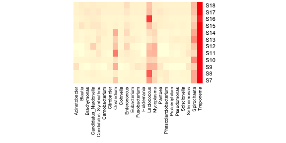 Much better! Now let’s add a dendrogram for the samples. The heatmap
function will do this for you, but I prefer to make my own using the
vegan package as it has more options for distance metrics. Also, this
means that you can do hierarchical clustering using the full dataset,
but only display the more abundant taxa in the heatmap.
Much better! Now let’s add a dendrogram for the samples. The heatmap
function will do this for you, but I prefer to make my own using the
vegan package as it has more options for distance metrics. Also, this
means that you can do hierarchical clustering using the full dataset,
but only display the more abundant taxa in the heatmap.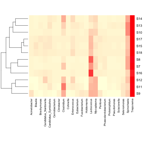 You can also add a column dendrogram to cluster the genera that occur
more often together. Note that this one must be done on the same
dataset that is used in the Heatmap (i.e. reduced number of genera).
You can also add a column dendrogram to cluster the genera that occur
more often together. Note that this one must be done on the same
dataset that is used in the Heatmap (i.e. reduced number of genera).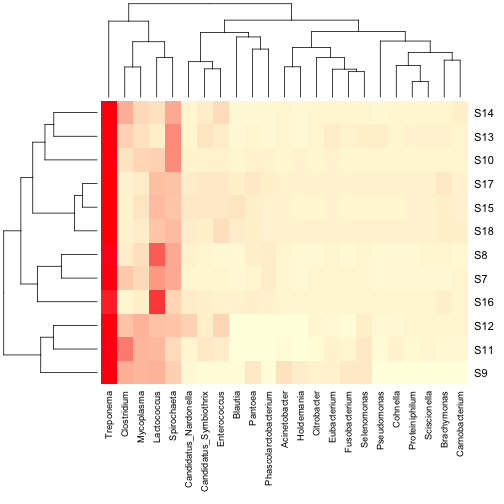 For some applications, the above heatmaps would be sufficient,
however, there are many times where it would be nice to indicate on the
heatmap values for other important variables, such as experimental
groups, or values of covariates. Also, it would be nice to have a legend
for the colour scale. heatmap.2 in the gplots package can do both of
these things.
For some applications, the above heatmaps would be sufficient,
however, there are many times where it would be nice to indicate on the
heatmap values for other important variables, such as experimental
groups, or values of covariates. Also, it would be nice to have a legend
for the colour scale. heatmap.2 in the gplots package can do both of
these things.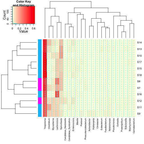 You’ll note that some of the defaults for heatmap.2 are kind of funny
looking. The green tracing in each column can be turned off with
You’ll note that some of the defaults for heatmap.2 are kind of funny
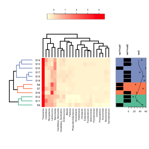
looking. The green tracing in each column can be turned off with 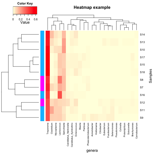 Finally, the least intuitive function is annHeatmap2 from the
Heatplus package. However, it allows for annotation with multiple
variables at once, as well as an option for colouring the dendrogram
into clusters. All of the options within the function are written as
lists, which can take some getting used to if you don’t use them
regularly.
Finally, the least intuitive function is annHeatmap2 from the
Heatplus package. However, it allows for annotation with multiple
variables at once, as well as an option for colouring the dendrogram
into clusters. All of the options within the function are written as
lists, which can take some getting used to if you don’t use them
regularly.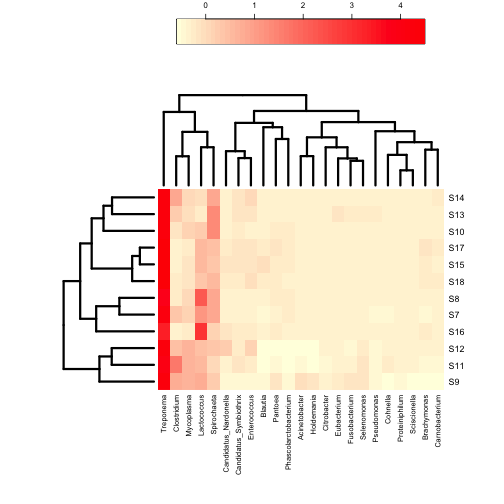 Annotations are added with the ann sublist which takes a data frame
as its input. Unlike the other functions, it can take multiple variables
for annotation including continuous variables.
Annotations are added with the ann sublist which takes a data frame
as its input. Unlike the other functions, it can take multiple variables
for annotation including continuous variables.
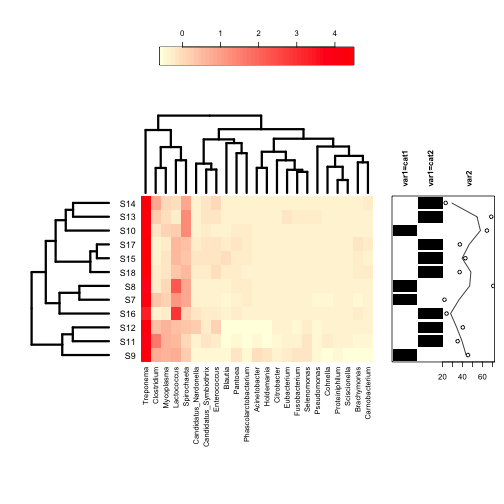 Finally, clusters in the dedrogram(s) can be highlighted using different colours with the cluster sublist: